5. Ionospheric Pierce Points (IPP) Map
This function considers both spatial and temporal domains, using the Ionospheric Pierce Point concept to represent the ISMR data according to the declared parameters on a map, projecting the IPP path over the selected time interval using aggregation methods.
After selecting the initial parameters, such as the time interval, the user can set as output parameters:
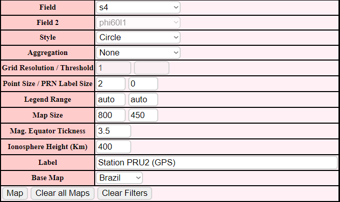
Figure 5.0.1 - Inputs
5.1 Field
Here the user selects the field that will be considered when generating the map along with the custom filters chosen earlier.
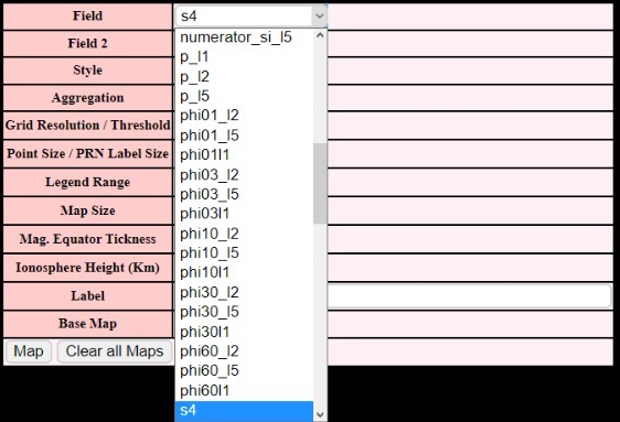
Figure 5.1.1 - Fields
5.2 Style
Define how the points will be displayed on the map
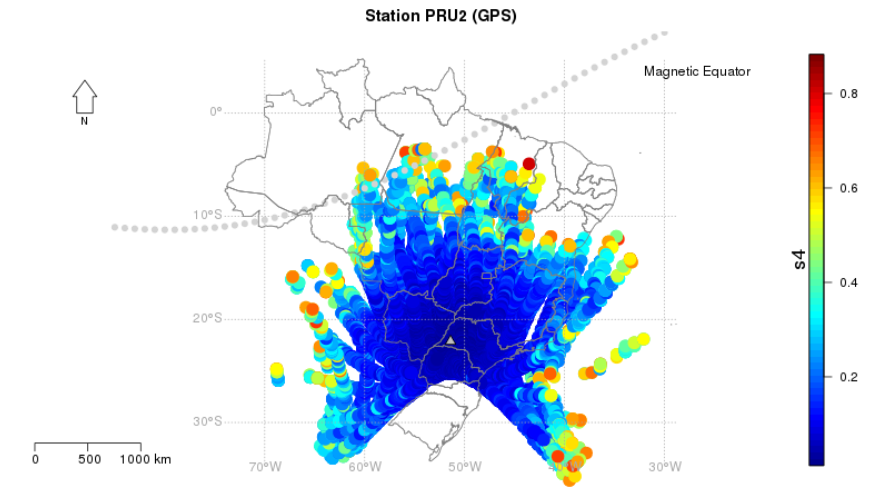
Figure 5.2.1 - Circle
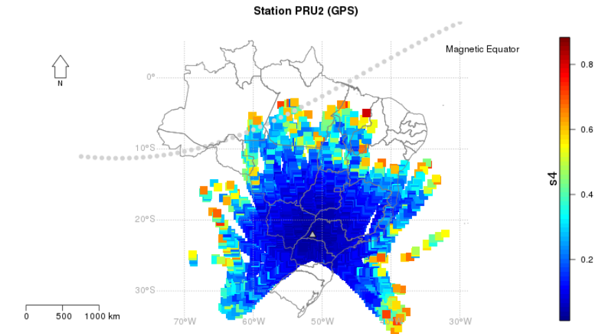
Figure 5.2.2 - Square
5.3 Aggregation
Aggregation consists in a way to summarize a comprehensive dataset using specific methods.
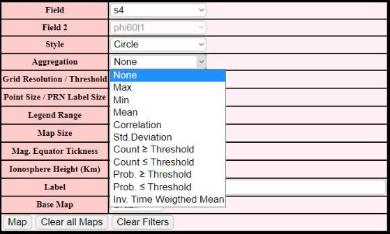
Figure 5.3.1 - Aggregations
Examples:
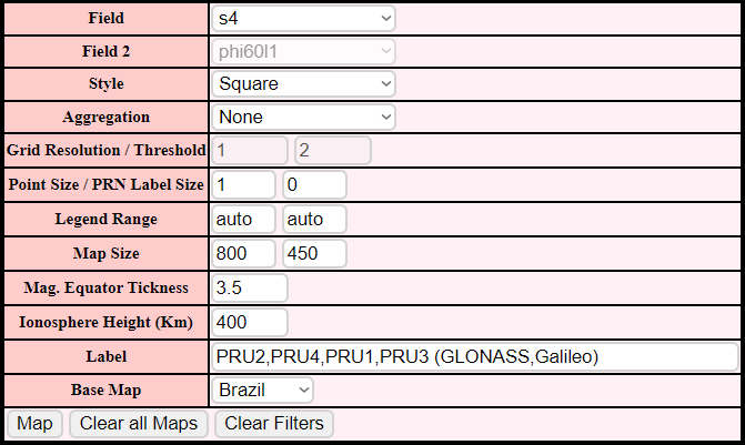
Figure 5.3.2 - Inputs
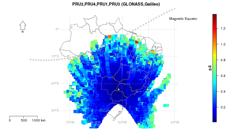
Figure 5.3.3 - Output
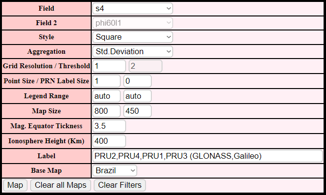
Figure 5.3.4 - Inputs
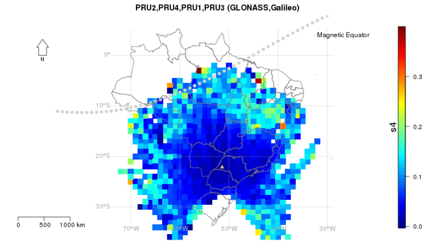
Figure 5.3.5 - Output
5.4 Grid Resolution / Threshold
Projection IPP Resolution according to the aggregation selected.
5.5 Point Size / PRN Label Size
-
Point Size:
Size of the displayed points
-
PRN Label Size:
Display size of the Pseudorandom number of the satellite from which the data was collected
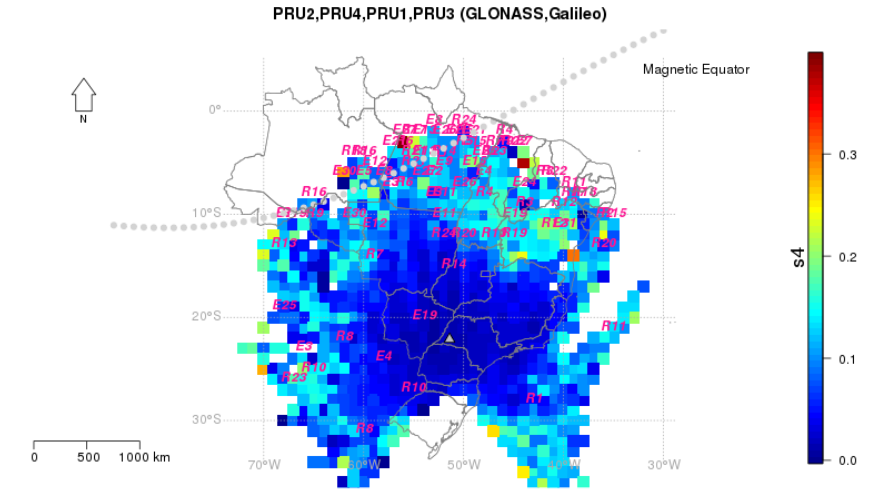
Figure 5.5.1 - Example with PRN Label Size as 1
5.6 Legend Range
Defines the range of values collected for the selected field that will be indicated by the legend
Example:

Figure 5.6.1 - Inputs
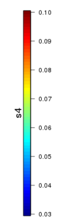
Figure 5.6.2 - Output
5.7 Map Size
Map size in the output (Width x Height)

Figure 5.7.1 - Input
5.8 Magnetic Equator Tickness
Defines the Tickness of the line that represents the Magnetic Equator in the map

Figure 5.8.1 - Input
5.9 Label
Name that will be displayed on the top of the map

Figure 5.9.1 - Input